Regression and Classification in ML (Machine Learning)

What is Regression in Machine Learning?

• Regression in machine learning involves predicting a continuous output or numerical value.
• In simpler terms, it's like estimating a quantity.
• Evaluation: Mean Squared Error (MSE), R-squared, etc
• Examples of Algorithms : Linear Regression, Ridge Regression, lasso Regression.
• For example, predicting house prices based on features like size, number of bedrooms, and location is a regression task.

Classification in Machine Learning

• Classification, on the other hand, is about assigning items into predefined categories or classes.
• Instead of predicting a continuous value, the algorithm categorizes input data into distinct groups.
• Evaluation : Accuracy, Precision, Recall, F1 Score and Confusion Matrix.
• Examples of Algorithms Support Vector Machines, Decision Trees, etc.
• For instance, classifying emails as spam or not spam, or identifying whether an image contains a cat or a dog.
• classification involves training a model to recognize patterns that define different classes
• , and then using those patterns to assign new, unseen data to the correct category.

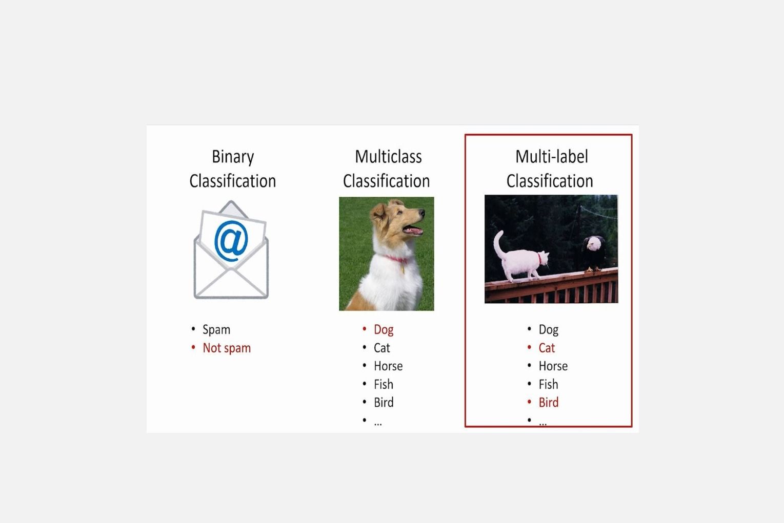
Binary Classification in Machine Learning

• Binary classification is a type of machine learning task where the goal is to categorize input data into one of two possible classes or categories.
• It's like making a yes/no decision, true/false prediction, or putting things into one of two boxes.

• Imagine you're building a spam filter for emails.
• The two classes in this scenario are "spam" and "not spam" (ham).
• The algorithm learns from labeled examples of emails – some marked as spam and some as not spam.
• After training, when you give it a new, unseen email, it predicts whether it belongs to the "spam" category or the "not spam" category.

Multiple Classification in Machine Learning

• Multiple classification, also known as multiclass classification, involves categorizing input data into more than two classes or categories.
• Instead of making a binary decision (yes/no, spam/not spam),
• the algorithm is trained to recognize and assign input data into several distinct categories.
• Each instance belongs to one and only one class.
• Clear decision boundaries separating classes.
• Example: Handwritten Digit Recognition
• Consider the task of recognizing handwritten digits from 0 to 9.
• This is a multiclass classification problem because there are multiple classes (0, 1, 2, ..., 9).
• The algorithm is trained on a dataset containing examples of each digit.
• After training, when you present it with a new handwritten digit, the model predicts which digit it is.

Multilabel Classification in Machine Learning

• Multilabel classification is a type of machine learning task where each input can belong to multiple classes simultaneously.
• In other words, instead of assigning just one label or category to each piece of data,
• Each instance can be associated with multiple labels simultaneously.
• Overlapping or shared decision boundaries as instances may belong to multiple labels.
• the algorithm can assign multiple labels, indicating that the input belongs to multiple categories at the same time.
• Example: Topic Tagging for Articles
• Consider a scenario where you have a collection of articles, and each article can be about multiple topics such as science, technology , etc.
• In a multilabel classification system, an article discussing both science and technology would be assigned labels for both categories.

Confusion Matrix in Machine Learning

• A confusion matrix is a table that helps evaluate the performance of a machine learning model, especially in classification tasks.
• It provides a comprehensive breakdown of the model's predictions by comparing is to the actual outcomes.

Components of a Confusion Matrix:

True Positives (TP):

• Instances where the model correctly predicts the positive class.
• Example: The model correctly identifies 50 spam emails.

True Negatives (TN):

• In this model correctly predicts the negative class.
• Example: The model correctly identifies 100 non-spam emails.

False Positives (FP):

• Instances where the model predicts the positive class incorrectly (false alarm).
• Example: The model incorrectly classifies 10 non-spam emails as spam.

False Negatives (FN):

• Instances where the model predicts the negative class incorrectly (miss).
• Example: The model misses 5 actual spam emails.

Usefulness of Confusion Matrix:

Accuracy

Precision

Recall (Sensitivity)

• Recall, also known as sensitivity or true positive rate, is the ratio of correctly predicted positive observations to all actual positives.
• A high recall indicates that the model is capturing a large proportion of the actual positive instances.

1# Assume True Positives (tp) and False Negatives (fn) are calculated or obtained
2tp = 120
3fn = 20
4
5# Calculate Recall
6recall = tp / (tp + fn)
7
8print(f"Recall: {recall}")

F1 Score

• The F1 score is the harmonic mean of precision and recall, providing a balance between the two metrics.
• To calculate accuracy using a confusion matrix, you can use the following

1# Assume precision and recall are calculated or obtained
2precision = 0.85
3recall = 0.75
4
5# Calculate F1 score
6f1_score = 2 * (precision * recall) / (precision + recall)
7
8print(f"F1 Score: {f1_score}")

Trade-off between Precision and Recall:

High Precision, Low Recall:

High Recall, Low Precision:

ROC Curve

• The Receiver Operating Characteristic (ROC) curve is a graphical representation.
• It illustrates the performance of a binary classification model across different thresholds.
• It is particularly useful when evaluating the trade-off between the true positive rate (sensitivity or recall).

Linear Regression with One Variable

• Linear regression with one variable, also known as simple linear regression,
• It is a basic method for predicting a dependent variable based on a single independent variable.
• Linear regression with one variable aims to find a straight line that best fits the relationship,
• between the independent variable (X) and the dependent variable (Y).

1Y= mx+b
2

Linear Regression with Multiple Variables

• Linear regression with multiple variables is an extension of simple linear regression,
• where instead of just one independent variable (x), we have multiple independent variables (x1​,x2​,...,xn​).
• This allows us to consider more factors that may influence the dependent variable (y).

Logistic Regression

• Logistic regression is a type of machine learning algorithm used for classification tasks.
• Unlike linear regression, which predicts a continuous output,
• logistic regression predicts the probability that an instance belongs to a particular category.
• Imagine predicting whether a student will pass (1) or fail (0) based on the number of hours they studied.
• Logistic Regression can output the probability of passing, and if it's above a threshold (e.g., 0.5), we classify it as a pass.

1. Binary Classification:

2. Probability Output:

• Instead of predicting a specific value, logistic regression predicts the probability that an instance belongs to the positive class.
• The output is between 0 and 1

1# Importing necessary libraries
2from sklearn.linear_model import LogisticRegression
3import pandas as pd
4from sklearn.model_selection import train_test_split
5from sklearn import metrics
6import matplotlib.pyplot as plt
7
8# Reading the dataset
9df = pd.read_csv("diabetes.csv")
10
11# Displaying information about the dataset
12print(df.info())
13
14# Splitting data into feature and target variables
15X = df.drop('Outcome', axis=1)
16y = df['Outcome']
17
18# Checking the label distribution
19print(y.value_counts())
20
21# Splitting data into training and test sets
22X_train, X_test, y_train, y_test = train_test_split(X, y, test_size=0.25, random_state=16)
23
24# Checking the label distribution in the test set
25print(y_test.value_counts())
26
27# Creating and training the Logistic Regression model
28logr = LogisticRegression(max_iter=1000)  # Setting max_iter to avoid warnings
29logr.fit(X_train.values, y_train)
30
31# Making predictions on the test set
32predicted = logr.predict(X_test.values)

Advanced Python

1. NumPy

• NumPy is a powerful Python library for numerical computing.
• It introduces a multidimensional array object (numpy array) that efficiently handles large datasets and
• provides a wide range of mathematical functions to operate on these arrays.

Pandas

• Pandas is a data manipulation library built on top of NumPy.
• It provides data structures like DataFrames, which are ideal for working with structured data.
• Pandas simplifies tasks like data cleaning, exploration, and analysis.

Scikit-Learn

• Scikit-Learn is a comprehensive machine learning library in Python.
• It provides tools for various machine learning tasks, including classification,
• regression, clustering, and more. It's built on NumPy, SciPy, and Matplotlib.

Conclusion